How high capacity utilisation hurts a team's performance
This is Beigel Bake, in Brick Lane, London.
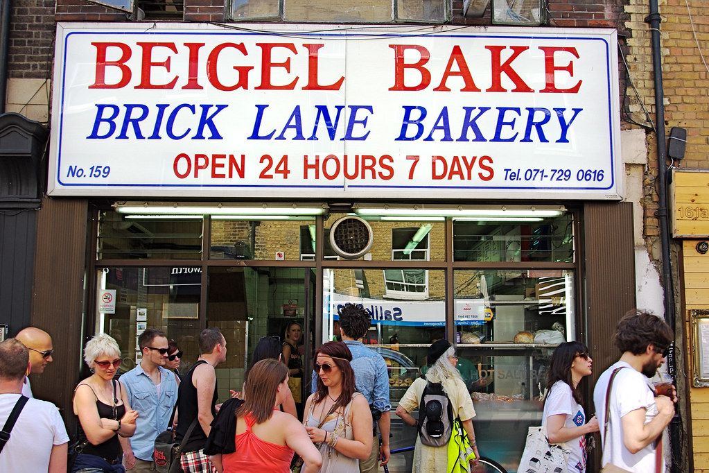
Beigel Bake is notorious for its salt beef beigels and humongous queues.
In this blog post, I'll use Beigel Bake to explain how capacity utilisation impacts queues and illustrate how queues hurt a team's performance. For that, I've written a few simple simulations to demonstrate how queues evolve over time and how capacity utilisation influences a queue's growth.
Then, I'll compare the beigel shop's queue to software development queues and expound on the similarities and differences between the two examples.
Finally, I'll present the alternatives for a software team to manage their queues, thus diminishing their economic impact and boosting the team's productivity.
The final part of this post summarises all the previous three.
In product development, our greatest waste is not unproductive engineers, but work products sitting idle in process queues.
— Reinertsen, Donald G. The Principles of Product Development Flow: Second Generation Lean Product Development.
The impact of queues
To decide whether you should join Beigel Bake's queue, there are two questions you could ask:
- How long did it take for the last customer to be served
- How long is the queue
Imagine you decide to take the first approach. In that case, you ask someone just leaving Beigel Bake: "how long did it take you to get a bagel?". "Ah, just two minutes", — they tell you.
Sweet! Two minutes for a mouth-watering salt-beef bagel? That's a deal worth taking.
Yet, after joining the queue, quite a few minutes go by, and you're nowhere near the counter. Why did that happen?
It happened because the person you asked joined the queue before you did. At the time, the queue was shorter. Therefore, they took less time to get to the front of the queue.
Someone that joined a 2-people long queue gets their beigel quite quickly. On the other hand, someone who enters a 20-people queue takes way more time to be served. In other words, the time it takes for people to get a beigel is a lagging indicator. It doesn't tell you anything about how long you will take to be served. That is, not unless you consider the length of the queue you're joining.
On the other hand, if you know twenty people are in front of you, and each beigel takes thirty seconds to prepare, you can estimate you'll take ten minutes to be served.
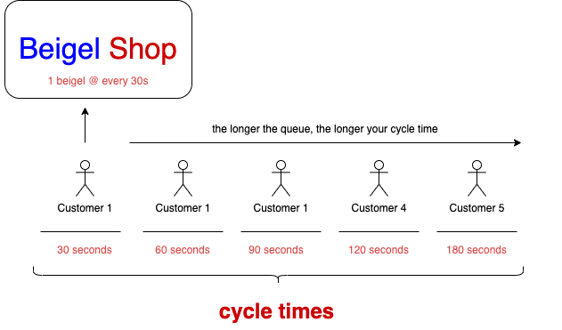
As you can see, Beigel Bake's queue size is a leading indicator of cycle-time — of how long it will take to get a beigel.
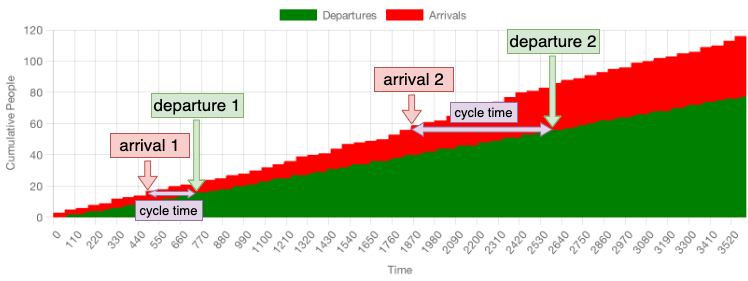
If you plot the cumulative number of customers leaving and arriving over time, the effect of queue sizes becomes easy to observe.
In the chart below, you can see that the rate of people arriving is greater than the rate of beigels served. Therefore, the shop's queue starts to grow, as evidenced by the difference between the cumulative number of arrivals and the cumulative number of departures, which represents the queue size.
Besides the queue's growth, the chart below demonstrates how customers joining a larger queue take longer to be served because they take longer to get to the front of the queue.
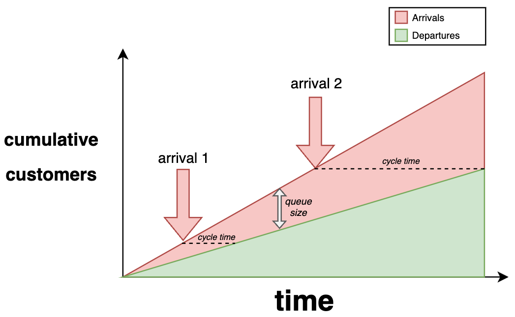
This type of chart is known as a cumulative flow diagram, or, in short, CFD.
In real life, most of us already follow this heuristic. If we see a massive queue, we're less likely to join it. Instead, we can decide to go do something else and come back later, when Beigel Bake is less busy.
By contrast, in software development, we often make the mistake of looking at how long it takes for each task to be done — a lagging indicator — instead of looking at the number of tasks we have to do — a leading indicator of total cycle-time.
When it comes to software, our queues easily become invisible because they're bytes on a hard-drive, not people on the sidewalk. That's why most engineers are blind to queue sizes but adamant about continuously measuring cycle-time and trying to diminish it.
The problem with trying to influence total cycle-time is that it is determined by how long your task queue is. The lengthier your queue, the longer your lead times (and cycle times) will be.
"But what is the problem with long lead times?" asks the perspicacious reader.
The first problem with lead times is that they amplify variability: the longer the lead times, the longer cycle times will get. That's because issues that join the queue later take longer to complete, even if they're as complex as another issue that joined earlier.
The second problem with long lead times is that they cause specifications to rot.
Imagine, for example, that you've written detailed stories for implementing a new discount coupon system for your online Beigel Shop. Three months later, when a developer finally picks up the coupon system's stories, it may be that they're not even worth implementing because you discovered customers are just as happy to pay the full price. Even in the best-case scenario, you'll have to revisit those stories to ensure the assumptions you've made at the time still make sense.
It's even worse when engineers implement these rotten specifications. In that case, they'll have spent time writing useless features which don't generate profit. Instead, each feature increases the software's bug surface, making it more expensive to maintain.
Either way, you've wasted time, effort, and money to create those specifications ahead of time.
Besides delaying feedback and producing economic waste, long queues demotivate engineers and make status reporting more complex, increasing management costs. Conversely, as queues get shorter, planning horizons shorten too. Consequently, we create more up-to-date specifications, which don't need as much rework and are more likely to generate profit because they have been made atop fresh pieces of information.
Furthermore, in case your customers don't like the new feature, shorter queues will allow you to start reworking it sooner.
Queues are the root cause of the majority of economic waste in product development.
— Reinertsen, Donald G. The Principles of Product Development Flow: Second Generation Lean Product Development.
Now that you understand the damages caused by queues, let's look at how queues behave so that we can diminish their impact.
Understanding a queue's behaviour
In this section, we'll simulate a queue's behaviour so that we can understand it. Then, we'll look at how to make queues smaller so that we can reap the economic benefits produced by shorter queues.
Beigel Bake has a single queue and, usually, two employees serving beigels. Each of those employees takes anywhere from one to two minutes to serve each beigel. On Sundays, when Beigel Bake is the busiest, one to three people join the queue each minute.
Using this data, we can write a program that simulates the queue's size over an hour. Our program will do the following:
- It will simulate one second at a time.
- Every second, arriving customers will be matched to a beigel server available.
- If no servers are available, the customer will join the end of the queue.
- Whenever a server delivers the customer a beigel, it will move on to serving the first person in the queue.
After the simulation finishes, the program will plot an area chart. This chart shows seconds on the X-axis, and the Y-axis tracks the cumulative number of customer arrivals, and beigels served.
Here's the result for one run of the simulation.
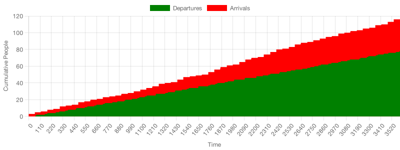
Similarly to the arrivals and departures chart I showed before, the vertical distance between the two bands represents the queue's size, and the horizontal distance between them represents cycle time. Just like before, as the queue grows, cycle-time grows too.
To diminish the time it takes for customers to be served, the beigel shop needs to reduce the vertical distance between the two bands.
For that, they must either:
- Increase the rate at which employees serve beigels
- Hire more servers
- Do both
Let's simulate option one and see what happens when we halve the time it takes for each employee to prepare a beigel.
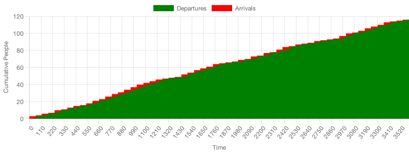
In this scenario, customers are more likely to find a free employee when they arrive because servers prepare beigels more quickly and free themselves up sooner.
Consequently, customers are less likely to find all servers busy and thus less likely to join the queue. In turn, the average queue length over time is smaller, reducing cycle times.
Now, let's simulate the second option. This time employees won't be as quick, but there will be twice as many employees working.
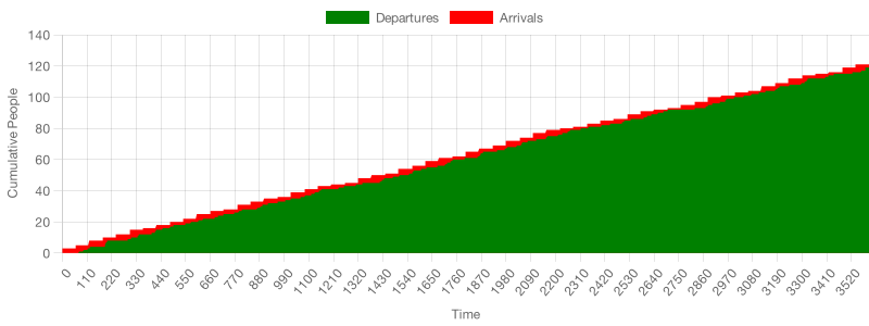
In this scenario, similarly to the previous one, there is barely anyone in the queue at any given moment. Because more employees are working, the likelihood of an arriving customer finding all servers busy is also smaller.
In both scenarios, there's one common factor which reduces queue formation: arriving customers are less likely to find all servers busy. That could be either because more servers are working or because servers are quicker and, therefore, free themselves up sooner.
This likelihood of finding all servers busy is influenced by one variable: capacity utilisation. Capacity utilisation represents the percentage of busy servers at a given time.
The more free servers, the smaller the capacity utilisation. As servers get busier, the capacity utilisation increases.
In the first simulation, where we saw queues forming, our average capacity utilisation throughout the simulation was 99%. The average capacity utilisation in the other two simulations was 72% and 77%, respectively.
That leads us to conclude that the more capacity we add, the less likely queues are to form. That's because customers are less likely to find all servers busy and, therefore, less likely to have to join a queue.
To summarise: at higher capacity utilisation levels, customers are more likely to find all servers busy and, therefore, join a queue.
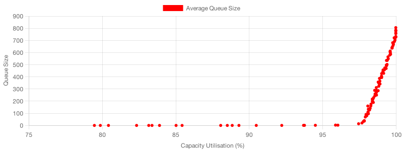
To see how our simulation behaves at different capacity utilisation levels, let's run this very same simulation (2 servers, 1 to 2 minutes per beigel) 100 times. For every time the simulation runs, we'll increase the number of servers, thus reducing capacity utilisation.
After all the simulations run, we'll create a scatterplot correlating the average queue size and the average capacity utilisation for each simulation.
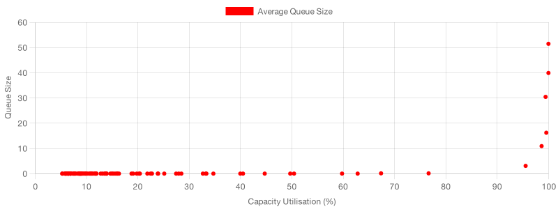
This scatterplot shows that the average queue size increases as the average capacity utilisation increases, just as we expected.
The effect of capacity utilisation in queue size can be even more apparent if we change our simulation's parameters and increase the rate at which people join the queue.
This time, we'll make eight to ten people join the queue every twenty seconds. That will diminish each server's impact on capacity utilisation, thus causing us to have more granular data at high utilisation levels.
There's yet a third lever the beigel shop could pull to diminish capacity utilisation: reduce the number of arrivals. However, that would not be a productive alternative in this case because it would decrease the shop's profit.
Finally, another important factor to notice in our simulations is that it wouldn't make sense to force spare capacity by asking a few employees to remain idle. If we were to do that, queues would still form because there would be fewer employees working. In these examples, the only ways to drive average capacity utilisation down were to make employees faster, increase the number of employees, or reduce the rate of arriving customers.
The beigel shop would only benefit from having spare employees if they were designated to serve high-paying customers, for example.
In that case, those high-paying customers would be happier because they would face shorter cycle times, but that would be at the expense of longer cycle times for other customers.
Queues and variability
As you've seen, when the beigel shop operates at high capacity utilisation levels, queues form. Therefore, if the shop's goal is to serve customers predictably, it must have excess capacity.
If the shop wanted to avoid having to have excess capacity, they'd only have one option: eliminate variability. Suppose every beigel takes the exact same amount of time to prepare and customers arrive at uniform intervals. In that case, the shop's owner can hire the precise amount of servers needed to produce beigels at the same rate customers arrive.
The cumulative flow diagram below illustrates what happens in a simulation where each customer arrives at a 30-second interval, and a single server always takes 30 seconds to prepare a beigel.
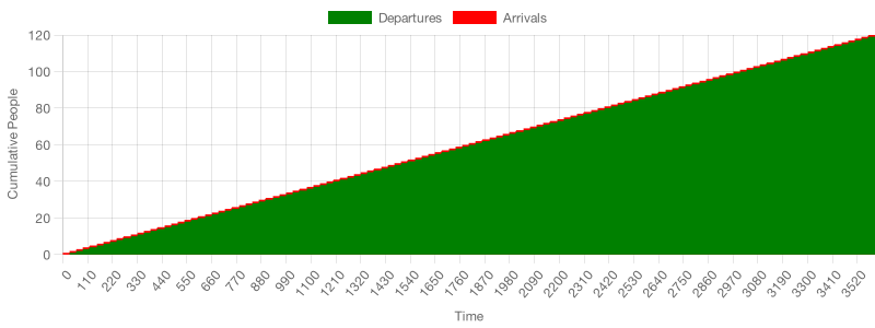
As the chart shows, when there's no variability and arrival rates match departure rates, there's no chance that the next customer will find all servers busy when they arrive.
In such a deterministic process, the server is always free when the next customer arrives. In this case, cycle times remain constant, and the queue size is always zero.
The problem with this approach is that most processes can't be made deterministic. In the real world, there is either elastic demand or variability in the time it takes for tasks to be done. Consequently, if we optimise for efficiency, that is, for keeping people busy, queues will form, and cycle times will sky-rocket.
That's the exact problem with Taylorism: it worships efficiency and thus allows for no spare capacity. This lack of excess capacity causes queues to grow, and, in turn, cycle time increases too.
Queue sizes, capacity utilisation and software development
Making the perfect salt beef beigel is complicated. So is making software. These two noble activities, however, also have plenty of notable differences.
In this section, I'll compare both examples and offer alternatives for better managing queues in software development.
Eliminating variability
The first obvious alternative to achieving predictable cycle times is eliminating variability in the time required to deliver tasks.
The problem with this option is that queues will continue to form if the team operates at 100% capacity. In that case, any arriving tasks would be queued.
Therefore, eliminating delivery variability would only be an option if you could also eliminate the variability of arrivals (the rate at which new tasks appear).
In the real world, none of these options is possible.
You can't eliminate variability in service times because software development is a stochastic process. The only way to know how long a task will take is to actually do it.
Eliminating variability in the rate at which tasks arrive is possible from a product perspective. In that case, you could simply create fewer tasks. You can't, however, write 100% bug-free software. Therefore, you'd have to assume that no one in your team will ever have to pick up an emergency or handle unforeseen events.
Adding excess capacity
Increasing the number of developers is the next obvious alternative for any team because more developers add capacity.
Although this option seems straightforward, it would only work if the extra developers bring capacity utilisation below 100%. Otherwise, queues would still form, and cycle times would still sky-rocket.
Imagine, for example, that you already have a long queue of tasks in your backlog. Because that queue of tasks is excessively long, developers are already always busy. In that case, adding an extra developer will only be helpful if it allows your long queue of tasks to come down to zero eventually. Otherwise, you'll remain at 100% capacity utilisation, and any new tasks will still go into the queue, increasing the variability of cycle times.
In other words, you'd have to sub-utilise resources to achieve predictable cycle times.
Although it's certainly possible to forcefully sub-utilise resources, it's challenging to do so.
For you to always have spare capacity, you'd have to allow a particular number of developers to remain idle so that they could respond to emergencies or surges in demand.
Alternatively, instead of having resources remain idle, you could explicitly allocate them to projects without deadlines. In that case, if a surge in demand happened, they'd drop their current work and address the incoming urgent activities. Some speculate that this is the reason for Google's 20% time, as explained here.
Please notice I'm not saying hiring more developers isn't helpful. Hiring more developers is beneficial because it allows you to ship more tasks. What I'm saying is that hiring more developers won't make your cycle times more predictable or diminish queues and their impact on your team's productivity.
Controlling queue sizes
In the beigel shop example, it would not be lucrative to impede customers from joining the queue as that would diminish the shop's profit. On the other hand, if you don't introduce queue limits to a software development process, it creates a vicious cycle of sky-rocketing cycle times, rotten stories, and frustration.
Imagine, for example, a team of engineers operating near maximum capacity. In that case, engineers must stop their current work to help refine the new tasks whenever new pieces of work come in. When engineers stop working on their current tasks, these tasks take longer.
Suppose there's no queue limit for this team. In that case, queues will continue to grow because every new batch of tasks not only increases the queue size but also delays the current tasks, which are already delayed because of the extra refinement work.
Then, when engineers get to implement the tasks they refined, those specifications will be more and more out-of-date each time, demanding even more rework and causing further delays.
On the other hand, teams that control queue sizes can operate at maximum capacity without significantly impacting their cycle time. That becomes possible because the time between creating stories and starting to work on them remains small.
Limiting queue sizes is one of the main reasons Kanban works so well. The work-in-process limits in a Kanban process ensure that items will only move from one stage to the next once the next stage has signalled it has enough capacity to pull in the next piece of work.
The differences between Beigels and Software
The arrivals and departures are significantly different between the two examples in this blog post.
For these examples, I've used uniformly distributed arrivals and departures. However, real-world queueing systems rarely see such a uniform distribution.
If you go study queueing theory, you'll see most people use Poisson arrivals and exponentially distributed processing times.
I've chosen not to do that in these examples for the sake of simplicity, as some of the same principles — the ones that matter for the topics I wanted to discuss — would still apply.
Putting it all together
The closer to 100% average capacity utilisation a system gets, the more likely it will be for new arrivals to go into a queue. As queues grow, lead times increase. Consequently, cycle times start sky-rocketing because teams will take incrementally longer to get to the queued tasks.
The longer a team takes to start a queued task, the more likely it is for its specifications to be out-of-date. These out-of-date specifications demand rework, which then delays other items in the queue even further.
Such a vicious cycle causes economic damage because it diminishes a team's productivity, makes its output unpredictable, and thus leads to decreased motivation, burnout, frustration, and poor financial results.
To make the most out of the resources available, you should control your queue's size and match the rate at which tasks are created to the rate at which tasks are finished. Systems whose queue size is limited have more predictable cycle times. Furthermore, this "just-in-time" approach to creating tasks decreases the likelihood of specifications rotting, hence boosting productivity and reducing rework.
Still, to deal with an inevitable surge in demand because of an emergency, there should be a certain margin of sub-utilisation to prevent queues from forming. Alternatively, managers could also look into hiring temporary extra capacity to deal with these spikes.
If I were to summarise this whole blog post's content in one piece of advice, that would be:
Instead of trying to control cycle times and capacity utilisation, focus on controlling your queues as they're the biggest source of waste in software development processes.
Related material
- A Dash of Queueing Theory — Tero Parviainen
- The most important thing to understand about queues — Dan Slimmon
- When efficiency hurts more than it helps — Dan Slimmon
- FAU Lectures on Queueing Theory — Prof. Robert B. Cooper
- Server utilization: Joel on queueing — John D. Cook
- Queues, Schedulers and the Multicore Wall — The Pith of Performance / Neil Gunther
Wanna talk?
You can book a call here. Really, that's it.
Alternatively, you can send me a tweet or DM @thewizardlucas or an email at lucas@lucasfcosta.com.
Subscribe
Get an email when I publish a new post. I'll never send you spam.
